梯度下降
梯度下降(随性的)
本文摘要
1.捏造一些用于拟合模型的数据
2.编写代价函数
3.编写梯度下降算法
捏造数据
因为手头没有数据,所以决定随机生成一批数据来进行拟合,因为存粹是尝试复现算法,所以姑且容忍这样射箭画靶子的行为。
1 | import random |

看起来还可以,蛮随机的
代价函数
$$
y=\theta_1x+\theta_2
$$
以上时我假定的一元回归模型,现在我们有一个模型,几个参数和一堆数据,对参数θ构建代价函数 J(θ)(cost function),通过求 J(θ)的最小值来求得最合适的参数。这个代价函数可以用离均平方和来计算
然后开始写我们的cost function
1 | def cost_function(theta1,theta2,data): |
可以了,完美,现在我们画画图看看
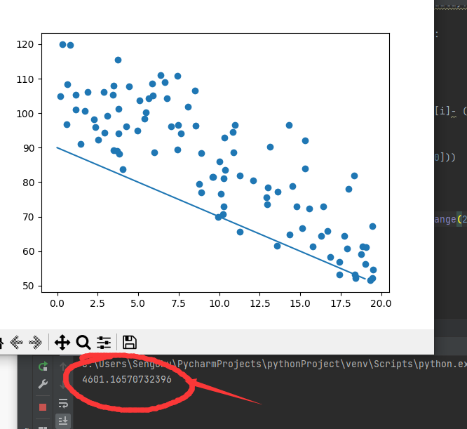
数据、模型、和代价函数,运行良好
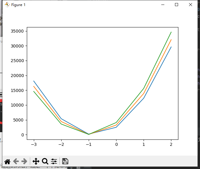
θ2为80、90、100时θ1的代价函数
梯度下降
梯度下降采用了一个逐步逼进的方法,选定一个下降率α,就可以逐步,慢慢的或者快快的得到我们最合适的参数
$$
\theta_1:=\theta_1-\alpha\frac{d}{d\theta_1}J(\theta1)
$$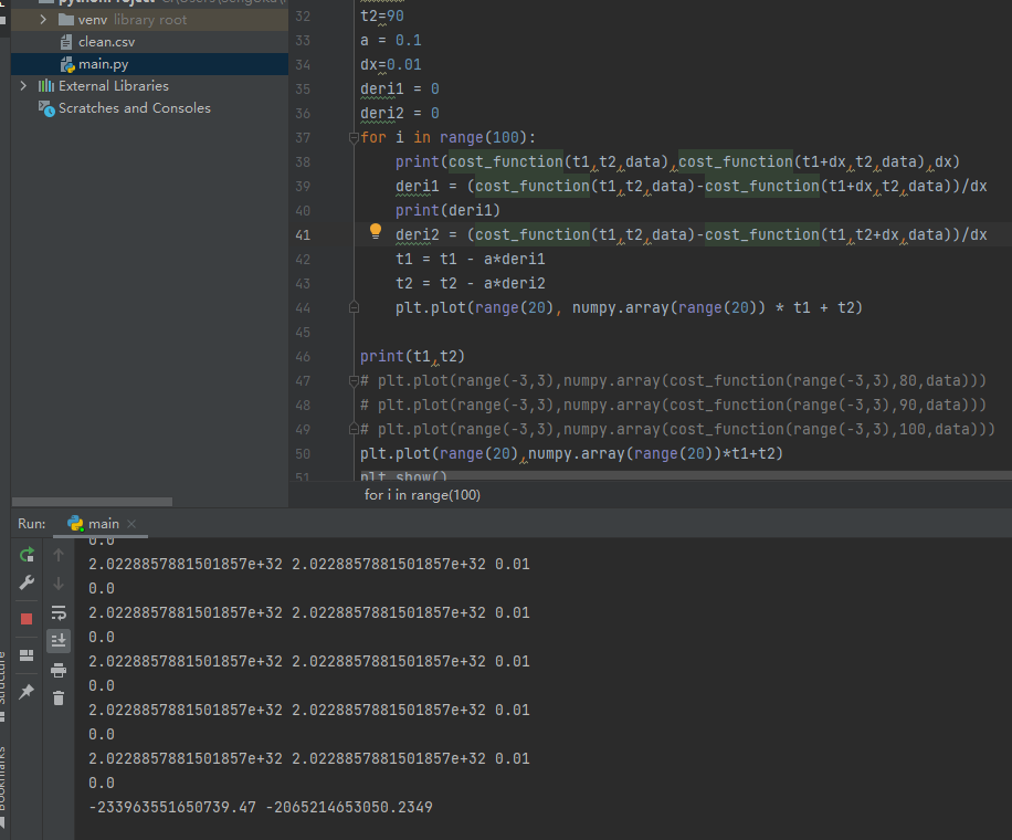
搓了一个,结果乱七八糟
经过十几分钟的尝试,终于找到了问题所在
1.α下降率设的太大了,我以为0.1是一个合适的值,但不是,太大了,直接飞出去了,导致参数爆了
2.没有做参数的标准化,两个参数插了两个量级….
其实在视频里早都提到了这两个问题,但是真的实践起来,还是和理论有些脱节的,一时间没想到,不过也好,这样理解相当深了
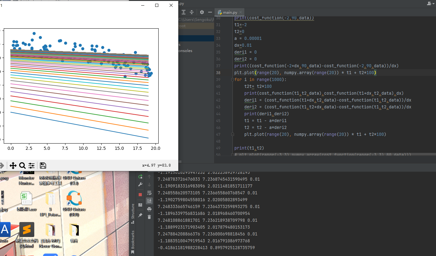
勉强跑起来的梯度下降
1 | t1,t2=-2,0 |
这是具体的梯度下降实现,下降率0.00001
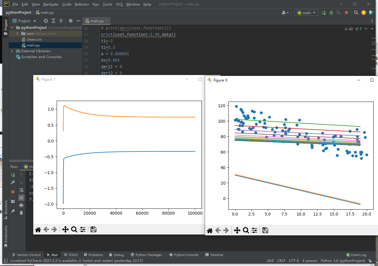
十万次迭代得到的极致模型
完整代码见下
1 | import random |